Making AI useful in the lab: the missing math of active learning

A call for greater first-principles theory to power lab-in-the-loop science

Before I begin, note that I am posting in a personal capacity and this blog does not represent any (official) positions of Relation. However, it does somewhat include reflections I’ve made from conversation with my talented colleagues! Andreas Kirsch was also involved in this work, but before his time at Google Deepmind.

---

There is enormous excitement for autonomous science: letting algorithms (or agents) control key aspects of experimental design to optimize the capability and capacity for inferring scientific truth. Naturally, this is most exciting when experiments are expensive and/or technically challenging to implement (e.g. single-cell sequencing) — which is basically all of the time if you’re doing anything in genomics.

Generally, I’ve seen two (not necessarily mutually exclusive) competing visions for autonomous science:

1. An LLM-centric view of the world trained via next-token prediction on scientific texts; entities (protein X, cell type Y, etc) are emergent phenomena. The model would then suggest future experiments to perform to resolve contradictions in the training data or build greater resolution over its world model.

2. An entity-based view of the world where variables defined a priori interact with each other — typically with error bars associated to these interactions. However, in most of biology, we do not know the underlying rules or parameters governing these interactions.

   1. In reinforcement learning (RL), we learn how act (a “policy”) by trial and error to maximise a reward in an environment with sequential decisions.

   2. If there are parameters to infer, then active learning (AL) is your tool of choice to learn a predictive model.

As I explained in an earlier post, the current “AI scientist” research arc appears to have a way to go before vision (1) is close to reality.

However, vision (2) is very much a reality… or is it? Whilst reinforcement learning is hugely popular, it is exceedingly data hungry, so nearly all of the applications relate to scenarios whereby one can computationally generate new data, e.g., AlphaGo.

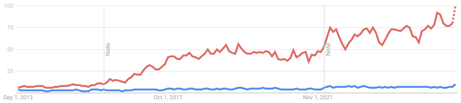
Active learning on the other hand never made it out of the starting gate (see Google Trends of RL in red vs AL in blue).

Active learning (AL) is concerned with how we improve the performance of predictive models by acquiring more training data: we require intelligent decisions about which data to acquire next, often in an iterative setting.

Virtually every conversation I’ve had about applying active learning (AL) in the real world with industry insiders ends with the premonition: it’s not worth your time, it will take years to get working, and acquiring data randomly is probably a safer option. My take on the reasons behind this is that:

1. There seems to be minimal mathematical justification behind some of the most simple and very popular algorithms.

2. Without such foundations, it is hard to model how the “real world” will undoubtedly break your base assumptions and the subsequent consequences thereof.

3. Therefore, no one has a strong understanding of how the marginal acquired data point relates to model error, and one cannot estimate how many experiments are actually needed to reach some acceptable tolerance.

In short, we are playing in the dark and we cannot expect AI to have a real impact on scientific discovery until we bottom this out.

Below, I give:

• Historical experience applying sequential model optimization

• My take on the field and how various ideas have been conflated

• The beginnings of a mathematical foundation for AL regression problems

---

Practice before Theory: The RECOVER Coalition

Go back to 2020: Relation had recently formed, COVID-19 had gone mainstream, and the Gates Foundation had announced their therapeutics accelerator. Seeing the announcement, we were lucky enough to work with the team at MILA and Turing prize winner Yoshua Bengio to put together a proposal (“RECOVER”) that received funding. The idea was simple: due to the challenges in understanding the mechanism of small molecule drugs in preclinical and clinical development and how drug-drug interactions occur, can we use AI to select pairs of drugs¹ that may work together to achieve an antiviral effect? This is a combinatorially difficult problem, if you have 10,000 drugs of interest, then you have ~50M pairwise drug combinations — completely infeasible to screen experimentally.

To achieve this, we created a deep learning model to predict how pairs of drugs impact an in vitro phenotype, set up wet-lab experimental systems to evaluate drug combinations, and then let the model choose pairs of drugs for evaluation. By performing this process iteratively, the idea was the model would identify increasingly efficacious drug combinations that human reasoning would not naturally put together.

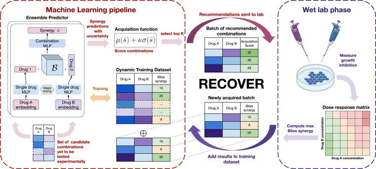
Building the deep learning models was challenging but achievable, the real difficulty was agreeing a strategy for how future drug combinations were selected. A common approach from AL was proposed, called “Least Confidence”, whereby we pose a collection (or “ensemble”) of deep learning models that each have slightly different versions of the training data, and subsequently see where they agree and disagree. If the models disagree, then conceptually the models are unsure about how some pair of drugs are going to work together, and in which case evaluating them experimentally and collapsing this uncertainty (typically referred to as “epistemic uncertainty”) should be highly informative to improve predictive accuracy.

At this stage, I started noticing a few key problems with the field. Notably, it was not clear how to deal with experimental replicates. Due to the instability of various cancer cell models we used during our proof-of-concept, we could run the same experiment 3 times and get 3 different (but similar) answers! For example…

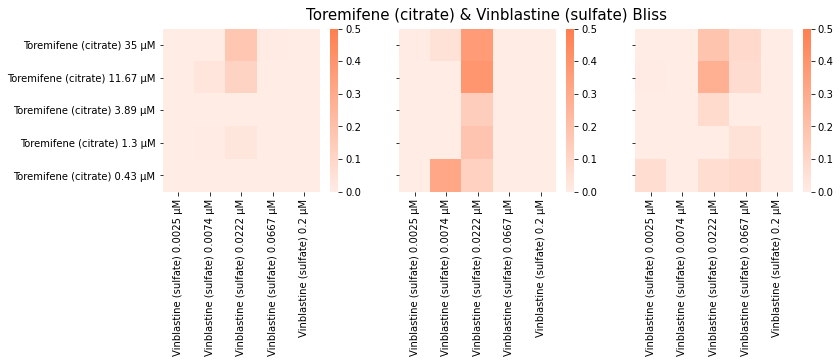
It occurred to me that if you’re trying to minimize model uncertainty (epistemic uncertainty), does this even make sense conceptually? The underlying process is noisy, so if a model is uncertain in some way, this may in fact be the correct inference.

To get around this (and noting that time was not on our side), there was a simple solution: skip trying to optimize for predictive accuracy, but to identify a different objective to optimize for. In our case, the objective became to find highly “synergistic” drug combinations (i.e., drug pairs that would be efficacious at low doses).² This way, we could move away from “vanilla” AL methods and use related approaches like Sequential Model Optimization (SMO) and/or Bayesian Optimization (BO), which are themselves built upon active learning principles. For the full write up, the associated publication is here.

Unfortunately, if you want to understand very complex biological or medical problems, there are rarely simple metrics that optimize for. In fact, no one has identified a quantifiable objective to suggest when an AI model actually understands biology — other than predictive accuracy! If you can make a highly accurate predictive model, then one can study the underlying structure of the model and try to assign meaning to it. In other words, if you don’t know the generating process for biology, then you have to infer it, and a necessary condition for the correct process is that it is predictive.

This does not however mean that an incorrect process cannot also predict the correct outcome, or that a model with substandard predictive power cannot capture the broad structure of the underlying biological process — but we don’t yet know many “core rules” of biological regulation beyond a few key motifs, e.g., signal transduction (ligand → receptor → downstream change, incl. TFs etc) and the central dogma of molecular biology (DNA → RNA → protein). So, if the field of active learning is about improving predictive accuracy, we really want it to work in practice!

---

Historical context

What is the core problem?

Fundamentally, our goal for active learning is to reliably outperform randomly designing future experiments, or “random selection”.

For a brief demonstration of how good random selection is, consider the following: we wish to estimate the area of a circle (because we have temporarily forgotten the formula due to selective amnesia, but in fact any shape would work). We can draw a circle inside a box, define a set of points that can be selected (e.g., consider the pixels on your computer screen), and then if you choose points at random, an estimate for the area of the circle is the proportion of points inside the circle multiplied by the area of the box; we call this Monte Carlo simulation. When compared to using a regular grid, random selection provides a much more accurate estimation of the circle’s area with the same number of points (on average — each realisation is of course different).

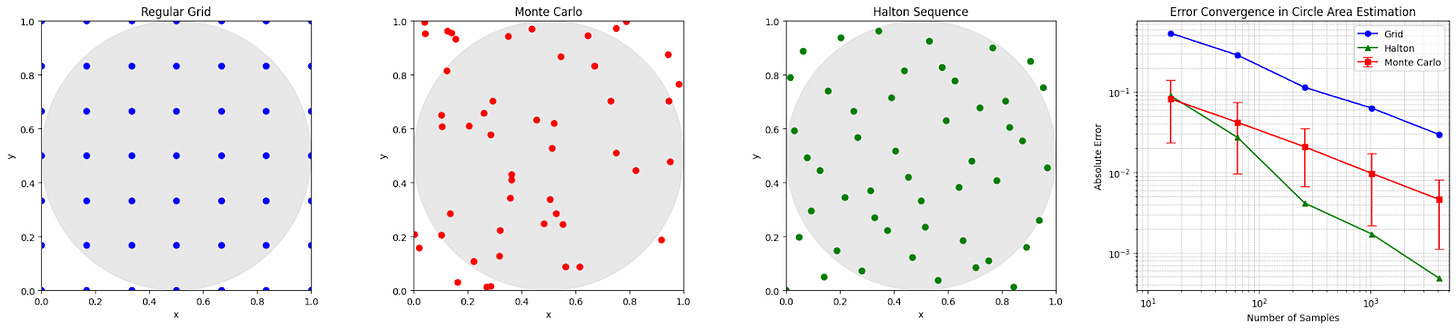
However, random selection can hypothetically be beaten: if you stop the randomly selected points from bunching too close together (e.g., via Halton sequence selection, which is deterministic), we build even more accurate estimates.

With Active Learning, a key weapon in our arsenal is that experiments can occur sequentially: we can select a point (or multiple points in a batch), assess its usefulness (however we define this), and then adjust our strategy accordingly.

A brief taxonomy of AL terms and state-of-the-nation

Most of active learning’s greatest hits were written for classification: pick the next image whose label (“cat”, “dog”, etc) you are most unsure about. The math and metrics lean on likelihoods and mutual information, but when people port these ideas to regression problems (the scientific setting where we care about quantities, e.g., concentrations, growth rates, binding affinities etc), the field gets confusing.

Here’s a classic example of a mismatch: Least Confidence.

• In classification it means that if there’s a low max-probability, then we assume that there’s a high “least confidence”:

  \(1-\max_c p_\theta\,(\,y\,{=}\,c\mid x)\)

• In regression it quietly morphs into “pick the largest predictive variance.” Same name, totally different quantity.

Before talking methods, a few working definitions:

• Epistemic uncertainty: model uncertainty that can shrink with more (or better-placed) data.

• Aleatoric uncertainty: measurement/process noise that won’t go away, no matter how much data you get. This quantity can be heteroskedastic and vary over the input space.

• Bias: the systematic gap between your model’s expected prediction and the truth.

All three are local quantities (they vary across the input space). You’ll often see high epistemic uncertainty where you’re far from training data; aleatoric spikes where the physics/assay is noisy; bias where your model class is just wrong.

To reason about real experiments, it helps to sort problems into three buckets:

Type I problems: Noiseless scenarios resulting from deterministic mappings (the simplest case).

For example, suppose you want to learn the relationship between Celsius and Fahrenheit: there is a direct relationship between the two defined by:

\(F = \frac{9}{5}C + 32\, .\)

These are typically very boring problems, and sadly a lot of AL benchmarking stops here.

Type II problems: Real-world scenarios with uncorrelated aleatoric noise, i.e., experiments are performed and we can essentially view all of them as independent and identically distributed (The “i.i.d” assumption).

Imagine we are trying to learn the dynamics governing various weather patterns from sensors located around the globe; each sensor may corrupt the true signal but we may wish to make the assumption that the functioning of one sensor is unrelated to the functioning of another, i.e., there are no correlations in the underlying noise process. However, this noise can still be heteroskedastic, e.g., we are better at quantifying slow wind speeds vs. fast wind speeds.

Type III problems: Real-world scenarios where aleatoric noise is correlated, i.e., we see systematic noise corrupting the whole system as we observe it.

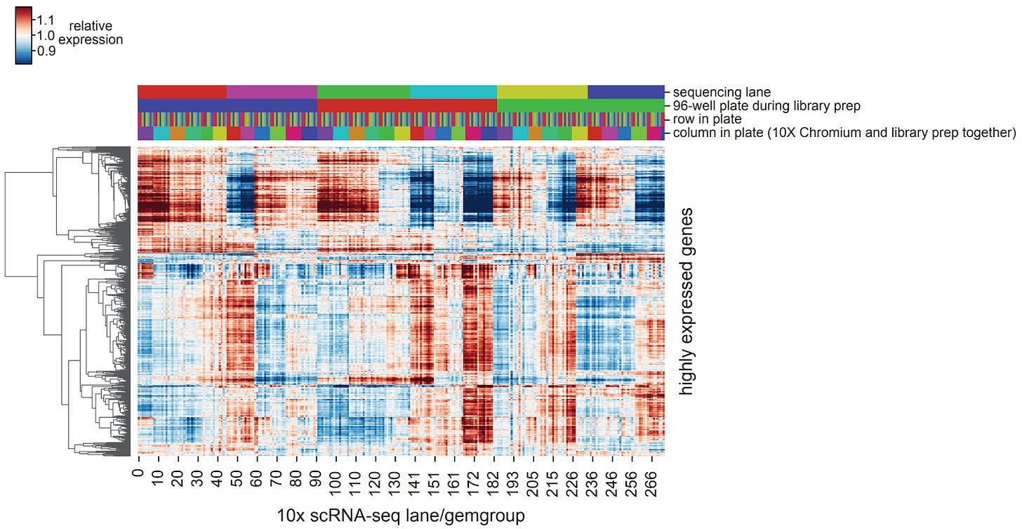
Consider the scenario where we’re running hundreds of experiments in parallel (e.g., cell growth assays) and the incubator temporarily shuts down and restarts without anyone noticing, then all of the cellular models in this batch all experienced the same random event, correlating the resulting experimental measurements. This is especially relevant to hot experimental systems biology techniques, e.g., pooled CRISPR screens with single-cell readouts (“perturb-seq”), whereby we see imperfections in the manufacturing process for microfluidic chips leading to systematic changes in gene expression measurements.

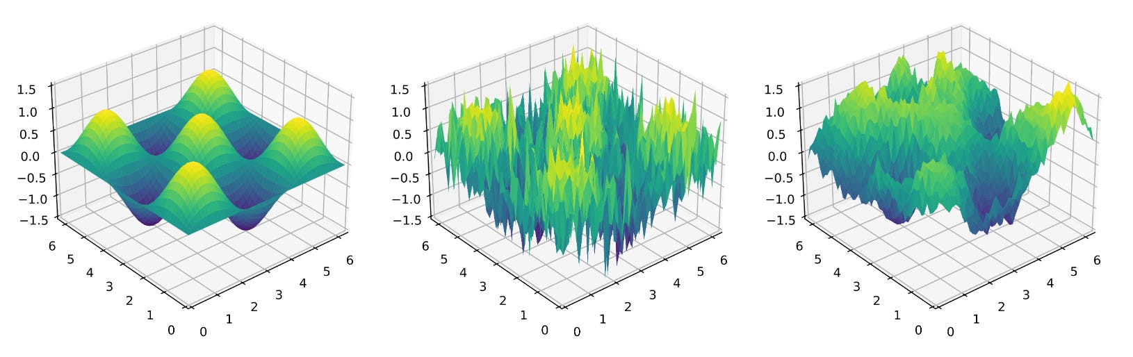
If you want to see versions of the same problem with different noise structures, see the two-dimensional function below: left is Type I (no noise), middle is Type II with independent noise for each (x,y)-coordinate, and right is Type III where (in this toy problem) the noise is similar in nearby regions of the state space.

To close, most AL theory is rock-solid only in narrow regimes (linear/GP models, i.i.d. homoskedastic noise, one-at-a-time querying). Add deep nets, batching, heteroskedasticity, correlated noise, or model misspecification, and the proofs thin out. Information-theoretic approaches (e.g., BALD) are principled in spirit, but with deep learning models they rely on approximations and can end up chasing irreducible noise. Net: foundations are solid in special cases; elsewhere we’re mostly dealing in heuristics plus empirical evidence. Scientific regression needs a cleaner story.

---

Towards a principled approach to AL

In our recent preprint, we start dealing with some of the above problems.

First, we note that for regression problems the bias-variance tradeoff can be applied and the expected mean squared error (EMSE) can be interpreted as the sum of an epistemic uncertainty term, the bias squared, and an aleatoric uncertainty term.³

One would ideally like to select points in the state space such that the bias is close to zero, but also that the predictive distribution approximately matches the underlying noisy oracle — we do not want our predictions being more or less certain than the underlying truth. Essentially, we cannot allow our predictive distribution (in purple) to be more confident than the underlying noisy process (in green):

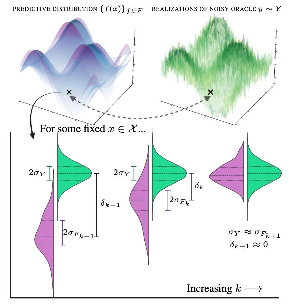
Naturally, when considering regions in the state space to select, some will correspond to areas whereby the bias or epistemic uncertainty rapidly collapses — and these should be prioritised for labelling when compared to the aleatoric uncertainty (that never changes)! We achieve this through calculating an approximation to the derivative of the EMSE between experimental rounds — leading to “difference” acquisition and our preprint title: two rounds of experiments can be used to estimate the gradient of the EMSE, which is then exploited in a third round of experiments (or indeed, any future experiments).

Finally, through noticing a mathematical trick, the bias-variance tradeoff can be adapted into a cobias-covariance tradeoff that allows for a neat way of proposing batches via eigendecomposition.

Recapping this in math-heavy language:

1. Target the right quantity. Decompose prediction error into

   \(\underbrace{\text{epistemic variance}}_{\text{shrinkable}} \;+\; \underbrace{\text{bias}^2}_{\text{shrinkable}} \;+\; \underbrace{\text{aleatoric noise}}_{\text{not shrinkable}}\)

   We call the sum of the first two the reducible error.

2. Estimate reducible error – not just uncertainty. Build a covariance-like operator over the pool:

   \(\Omega \;=\; \Sigma_F \;+\; \Delta \;+\; \Sigma_Y\)

   where ΣF​ is epistemic covariance (from an ensemble/GP), Δ=δδ⊤ captures bias via the co-bias matrix, and ΣY​ is aleatoric covariance (including batch correlations). Two practical tricks:

   • Difference acquisition: compare consecutive rounds so stationary ΣY​ cancels, revealing where reducible error is actually collapsing.

   • Quadratic estimation: predict entries of Δ directly (pairs), which is numerically more stable for batching than first predicting δ and squaring.

3. Batch smartly with eigenmodes. Work on the reducible operator

   \(\Omega^{\text{red}}=\Sigma_F+\Delta\)

   Take its top eigenvectors and, for each, pick the input with the largest loading. You end up spreading the batch across orthogonal directions of reducible error, not just piling into one noisy hotspot.

Why this is different to much of the previous literature:

• Optimizes the metric that matters. We explicitly target expected MSE, not a proxy for “uncertainty”. Such methods are referred to as “Expected Error Reduction” approaches.

• Separates signal from noise. The difference trick cancels stationary aleatoric terms; the cobias-covariance view makes correlated noise an explicit object you can model or subtract.

• Smarter batching by design. Eigenmodes give diversity: cover distinct, high-impact directions that reduce error after retraining (given various caveats about how well the underlying neural network can capture the underlying data).

• Model-agnostic but practical. Plays nicely with deep ensembles, MC-dropout, or GPs; no need for idealised assumptions to get started.

Ultimately, we are interested in designing algorithms for the messy realities of drug discovery and systems biology — replicates, batch effects, shared lab equipment, etc — and this is a small step on this journey.

1. This was posed as an alternative strategy to vaccines: the effect is immediate and you don’t need to wait for an adaptive immune response to form.

2. Drug synergy is the concept that one can lower doses and maintain the same effect by pairing therapeutic agents together that interact with complementary aspects of biology. For example, many HIV drugs are not in fact one drug, but a carefully blended cocktail of antivirals. There are a range of metrics to quantify this that leverage combinatorial dose-response screens; these metrics can be a optimized for by a machine learning model.

3. More general bias-variance tradeoffs exist through the use of Bregman divergences, so you can still use the same philosophy to deal with discrete problems too.